Understanding the Kullback-Leibler Divergence
How well can we fit a model to a set of real data? In this post we will understand the Kullback-Leibler (KL) divergence and its relationship with the maximum-likelihood optimization.
- All models are wrong, but some are useful
- Bits required to encode information: entropy
- Distances, Metrics & Divergences
- Relationship to the maximum-likelihood principle
- References
EDIT: This is a new version of a previously posted text, written back in 2017.
All models are wrong, but some are useful
Reality is, and always will be, far more complex than the models used to describe it. Therefore whenever we make use of a model, there will be a net loss of information. This means that in general such model will not be able to reproduce or reflect all the features and properties of the physical system under modeling.
This is particularly true in Statistics and Probability theory, where many times we seek to compare how close two probability distributions are. For instance, imagine a physical system that displays a probability distribution \(p\) whereas you are trying to model it by a set of parameters \(\theta\) whose outcome is another distribution \(q\). We aim at making q as similar to p as possible. In what follows we shall assume unidimensional distributions over \(x\) such that \(p = p(x)\) and \(q = q(x; \theta)\) with \(x \in \mathcal{X}\).
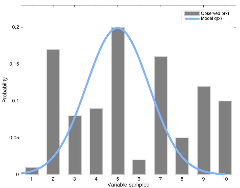 Fig. 1. Illustration of an observed distribution \(p(x)\) modeled by a Gaussian \(q(x;\mu, \sigma^2)\).
Bits required to encode information: entropy
In Information Theory, the concept of entropy is widespread almost everywhere. Although loosely related to the thermodynamic term, in this context we define it as:
\[H(p) = -\sum^N_{i=1} p(x_i)\log p(x_i) \text{ [discrete]}\] \[H(p)= - \int_x p(x)\log(x) dx \text{ [continuous]}\]where \(N\) denotes the number of elements or observations available from the system that yielded the probability density. In a general way, it can be written as:
\[H(p) = - \mathbb{E}_{x \sim p} \log(x)\]\(\mathbb{E}_{x \sim p}\) denotes the expected value when \(x\) is sampled from the probability distribution \(p(x)\). In Computer Science, the \(\log p(x_i)\) is usually \(\log_2 p(x_i)\), and it is a measure of the “minimum amount of bits needed to encode a piece of information”. You can think of it as a way to interpret how much information there’s within a system.
Similarly, the cross-entropy roughly points out the amount of information from a distribution \(p(x)\) that is encoded by anoter one \(q(x;\theta)\):
\[H(p, q) = -\sum_x p(x) \log q(x)\] \[H(p, q) = -\int_x p(x) \log q(x) dx\]Equivalently,
\[H(p, q) = -\mathbb{E}_{x\sim p}\log q(x)\]Distances, Metrics & Divergences
We aim at capturing the difference between two probability distributions. Probably the simplest way to get a flavour on how close two any distributions are is to compute a scalar value that grows greater with the difference between pairs of points of both distributions. Although we have defined it colloquially, what we are referring to is known as statistical distances.
Unfortunately, it is not strange at all to read scientific papers in which the authors use indistinctibly the distance (meaning statistical distance) and metric, although they are not the same. A metric on a set \(\mathbb{X}\) is a function
\[d: \mathbb{X} \times \mathbb{X} \rightarrow \mathbb{R}^+\]where \(\mathbb{R}^+\) is the set of non-negative real numbers such that for all \(x, y, z \in \mathbb{X}\), \(d\) satisfies:
- Non-negativity: \(d(x,y) \geq 0\)
- Identity of indiscernibles: \(d(x,y) = 0\) if and only if \(x = y\).
- Symmetry: \(d(x,y) = d(y,x)\)
- Triangle inequality: \(d(x,z) \leq d(x,y) + d(y,z)\)
Since statistical distances do not need to be symmetric, as a rule they will neither be, strictly speaking, metrics. Divergences are a special subset of statistical distances.
KL Divergence
The Kullback-Leibler Divergence \(D_{KL}(p\mid \mid q)\) belongs to the family of statistical distances known as f-divergences (Csiszár & Shields, 2004), and is defined as:
\[D_{KL}(p \mid \mid q) = \int_x p(x)\log p(x) dx - \int_x p(x) \log q(x) dx\] \[D_{KL}(p \mid q) = \int_x p(x) \log \frac{p(x)}{q(x)} dx\]which can also be written as
\[D_{KL}(p \mid \mid q) = \mathbb{E}_{x \sim p} \left[ \log p(x) - \log q(x) \right]\]which is easy to see is equivalent to
\[D_{KL}(p \mid \mid q) = H(p) - H(p,q)\]\(D_{KL}\) is thus but the difference between the entropy of the true probability distribution \(p(x)\) and the cross-entropy of \(p(x)\) and \(q(x; \theta)\). In short, we are measuring the information lost when using an artificial probability distribution \(q(x;\theta)\) to describe the true probability distribution \(p(x)\).
Its behavior
It is easy to see that if both \(p(x)\) and \(q(x;\theta)\) are well-defined, the KL divergence is always positive (non-negativity). However, it is not always simmetrical, nor is does it satisfy the triangle inequality. This means that the actual value of the KL divergence depends on the distribution from which we are measuring.
There is a couple of special cases, namely those related to the points in which one of the distributions takes a zero value:
- When \(p(x) = 0\), the \(\log\) is not defined, so the KL divergence is no longer a valid measure. It is not defined at one point at least, so a walk-around is to add some noise to the original data distribution, ensuring that \(p(x) > 0\) everywhere.
- If \(q(x) = 0\) and \(p(x) > 0\), \(p(x) / 0 \rightarrow \infty\). In other words, if there’s no \(q(x)\) in a place it was supposed to be, the distance between probability distributions becomes infinity.
Relationship to the maximum-likelihood principle
If you use to read machine learning research papers, it is very likely that you have already come accross the notion of maximizing the maximum-likelihood, or equivalently, minimizing the negative log-likelihood. Most of our deep neural methods nowadays are trained following this scheme (Goodfellow et al, 2016).
Through this procedure, neural networks learn to progressively reduce the gap between their inner model (which we might identify with \(P_\theta(x)\)) and the real distribution \(\hat{P}_D(x)\) of the observed data. In short, an iterative process over the parameters \(\theta\) works to make \(P(x;\theta) = P(x \mid \theta) = P_\theta(x)\) closer to \(\hat{P}_D(x)\).
Learning by observing
Let us denote by \(\hat{P}_D(x)\) the probability of an instance in a dataset:
\[\hat{P}_D(x) = \sum_{i=1}^N \frac{1}{N}\delta_(x-x_i)\]From the definition of KL divergence
\[D_{KL}(\hat{P}_D(x) \mid \mid P_\theta(x)) = \int_x \hat{P}_D(x) \log \frac{\hat{P}_D(x)}{P_\theta(x)} dx =\] \[= -H[\hat{P}_D(x)] - \int_x \hat{P}_D(x) \log P_\theta(x) dx\]when deriving the gradient of the above expression with respect to \(\theta\),
\[\nabla_\theta(D_{KL}(\hat{P}_D(x) \mid \mid P_\theta(x))) = \nabla_\theta \mathbb{E}_{\hat{P}_D(x)} \log P_\theta(x)\]since \(\hat{P}_D(x)\) is independent of \(\theta\). If we continue expanding the expression above,
\[\nabla_\theta \sum_x \hat{P}_D(x) \log P_\theta(x) =\] \[\nabla_\theta \sum_x \left[ \frac{1}{N} \sum_{i=1}^N \delta_(x-x_i) \right] \log P_\theta(x)\]and therefore
\[\nabla_\theta(D_{KL}(\hat{P}_D(x) \mid \mid P_\theta(x))) = \frac{1}{N} \sum_x \nabla_\theta \log P_\theta(x)\]And here we are, at a completely analogous expression to that of the original log-likelihood problem! This is a very important result, since it assures us that when our learning systems are training under a negative log-likelihood strategy, they are actually learning to match the distribution as seen in the dataset.
The importance of fundamentals
In fact, this topic has attracted a lot of attention in recent years due to the rising of Generative Adversarial Networks (Goodfellow, 2016) and Variational Autoencoders (Doersch, 2016). Both types of models try to estimate the difference between two densities. Researchers in this area have came up with new statistical distances, some of them being also metrics; I find particularly interesting the Wasserstein GAN (Arjovsky, 2017) and the Cramér GAN (Bellemare et at., 2017) papers. Sadly, these are heavy stuff thet I hope to cover in further posts.
References
Arjovsky, M., Chintala, S., & Bottou, L. (2017): “Wasserstein GAN”. arXiv:1701.07875
Doersch, C. (2016): “Tutorial on Variational Autoencoders”. arXiv:1606.05908
Goodfellow, I. (2016): “NIPS 2016 Tutorial: Generative Adversarial Networks”. arXiv:1701.00160
Goodfellow, I., Bengio, Y. and Courville, A. (2016); “Deep Learning” MIT Press (Online).